1. Introduction

During a drought, a regulator may need to limit how much water a community can use. One way to do this is through a tradable water permit system.

The regulator sets a fixed cap on total water use and distributes permits to households. One permit allows a household to consume one gallon of water.

Households can then trade these permits:

• A household that values additional water more can buy permits.
• A household that values additional water less can sell unused permits.
• The market price helps coordinate these decisions under the fixed water cap.

Tradable water rights are not only a theoretical idea. Water markets have been used in countries including Australia, Chile, and the United States, although their design and performance vary. Their success depends on institutions such as clearly defined rights, reliable measurement, trading rules, and effective oversight ^[1].

Hu et al. developed an urban water-permit framework in which residents could sell conserved water to industrial users using smart-meter data. Our simulation uses a related idea, but it focuses on trading between households and removes most institutional and technological details ^[2].

The goal of this simulation is to design the simplest theoretical model that explains:

1. how a household chooses its water consumption.
2. how permit demand changes with price.
3. how a market-clearing price is found.
4. which households buy or sell permits.

We are going to assume that households are rational, all trades occur at one common price, permits and water are continuously divisible, and permits are perfectly enforced. The model also excludes transaction costs, income constraints, uncertainty, and strategic behavior.

---

2. Why allow households to trade?

Suppose every household $H_i$ receives the same initial number of permits. And each household has different water-valuation parameters $A_i$. This is simply a number that represents how strongly $H_i$ values water.

An equal allocation may appear fair, but there's a problem with this system where it creates an economic inefficiency. At the same level of consumption, one household may receive a larger benefit from an additional gallon than another household.

For example, suppose $H_A$ and $H_B$ receive the same number of permits. If $H_A$ places more value on one additional gallon than $H_B$, transferring one permit from $H_B$ to $H_A$ can increase the total benefit produced by the fixed water supply.

A more practical example is a large household may need more water for drinking, cooking, and hygiene. Another household may have fewer members or lower water needs.

Without exchanging permits, one household may have unused permits while another lacks water for more valuable uses. Later, we will call the value of one additional gallon its marginal benefit. In theory, trading allows permits to move from households with a lower marginal value of water toward households with a higher marginal value ^[3].

Under competitive markets, clearly defined rights, complete information and low transaction costs, this can increase the total benefit produced by a fixed water supply. These conditions are important: trading does not guarantee an efficient result when they are absent.

---

3. Modeling how a household values water

Let household $i$'s water consumption be:

$$q_i \geq 0$$

where $q_i$ is measured in gallons.

We represent the household's benefit from water using a logarithmic utility function:

$$U_i(q_i)=A_iln(q_i+1)$$

where:

• $q_i$ is the household's water consumption.
• $A_i$ is the household's water-valuation parameter.
• $U_i(q_i)$ is the household's total benefit from consuming water.

A higher $A_i$ means the household places more value on water. A household may first use water for drinking, cooking, and basic hygiene. While additional water may then be used for less urgent activities. This does not mean households literally consume water in that exact order. It means that when water is scarce, households are expected to allocate it toward their most valuable uses first.

We choose the logarithmic function because it is simple and has two useful properties:

$$U_i'(q_i) > 0$$

so additional water increases total benefit, and:

$$U_i''(q_i) < 0$$

so the benefit added by each additional gallon becomes smaller.

The logarithmic form is a modeling assumption, not a claim that it perfectly describes real households. Utility maximization is a standard starting point for household water-demand models, but this paper deliberately uses a simplified functional form ^[4].

For simplicity, we measure $U_i(q_i)$ in money-equivalent units. This allows the benefit of water to be compared directly with the monetary price of a permit.

---

4. The marginal benefit of water

Marginal benefit is basically the maximum amount a consumer is willing to pay for one additional unit of a good or service, or the extra satisfaction (utility) gained from it.

To find the marginal benefit, we take the derivative of the utility function. A derivative measures how much one variable changes when another variable increases slightly. In this case, it tells us how much the household's total utility changes when water consumption increases by one additional gallon.

Therefore:

$$MB_i(q_i)=\frac{dU_i(q_i)}{dq_i}$$

Substituting the utility function, we get:

$$\frac{dU_i(q_i)}{dq_i}=\frac{d(A_iln(q_i+1))}{dq_i}$$

Using the derivative rule, we get:

$$\frac{d(A_iln(q_i+1))}{dq_i}=\frac{A_i}{q_i+1}$$

Therefore:

$$MB_i(q_i)=\frac{A_i}{q_i+1}$$

For example, suppose $H_A$ has:

$$A_A=1000$$

and $H_A$ currently consumes:

$$q_A=100$$

Then the marginal benefit of $H_A$ is:

$$\begin{aligned} MB_A(100) &= \frac{1000}{100+1} \\[0.75em] &= \frac{1000}{101} \\[0.75em] &\approx 9.90 \end{aligned}$$

Therefore the 101st gallon provides approximately $9.90$ units of additional benefit. But if the household already consumes $900$ gallons of water, then:

$$\begin{aligned} MB_A(900) &= \frac{1000}{900+1} \\[0.75em] &= \frac{1000}{901} \\[0.75em] &\approx 1.11 \end{aligned}$$

Therefore the 901st gallon provides approximately $1.11$ units of additional benefit.

The 101st gallon is more valuable than the 901st gallon because the household already has much more water in the second case.

---

5. Comparing water benefits with the permit price

A household does not decide how much water to use based only on how useful water is. It must also consider the cost of obtaining permission to use that water.

In this market, every additional gallon requires one additional permit. Even if a household already owns the permit, using it still has an economic cost because the household could have sold it instead. This is called an opportunity cost.

The household therefore compares two things:

• The benefit of consuming one more gallon of water;
• The market value of the permit needed for that gallon.

For simplicity, we interpret utility in money-equivalent units. This means that the marginal benefit of water can be compared directly with the permit price.

Let:

$$p > 0$$

represent the market price of one water permit.

With the comparision, we can derive a decision rule where the households:

$$\begin{aligned} MB_i(q_i) > p &\quad\Rightarrow\quad \text{consume more water},\\ MB_i(q_i) < p &\quad\Rightarrow\quad \text{consume less water},\\ MB_i(q_i) = p &\quad\Rightarrow\quad \text{stop adjusting}. \end{aligned}$$

The optimal economic condition is where:

$$MB_i(q_i)=p$$

Substituting the marginal-benefit equation gives:

$$\frac{A_i}{q_i+1}=p$$

This is the optimal economic condition, where household consumes water until the value of its final gallon equals the market price of a permit.

---

6. Solving for household water demand

The previous section gave us the household's decision rule. We now want to turn that rule into a demand function. A demand function tells us how much water a household wants to consume at a given permit price.

This is useful because the market price may change. When permits are cheap, households are likely to consume more water. When permits become expensive, households have a stronger incentive to conserve water.

We begin with the household's optimal condition:

$$\frac{A_i}{q_i+1}=p$$

Now solve for $q_i$:

$$\begin{aligned} A_i &= p(q_i+1),\\ \frac{A_i}{p} &= q_i+1,\\ q_i &= \frac{A_i}{p}-1. \end{aligned}$$

So household $i$'s demand for water is:

$$q_i^*(p) = \frac{A_i}{p}-1$$

Since water consumption cannot be negative, we can rewrite $q_i^*(p)$ as:

$$q_i^*(p) = \max \left\{{\frac{A_i}{p}-1, 0}\right\}$$

The star in $q_i^*$ means that this is the household's optimal level of water consumption at price $p$.

The resulting demand function is intended to illustrate the economic mechanism. It has not been calibrated using observed household water-consumption data. A more realistic simulation would estimate or calibrate its parameters using empirical water-demand elasticities ^[5].

The demand function gives us two important relationships. If the household values water more strongly, its demand rises:

$$A_i \uparrow\Rightarrow q_i^*(p)\uparrow$$

If the permit price rises, its demand falls:

$$p \uparrow\Rightarrow q_i^*(p)\downarrow$$

So households with higher water-needs tend to demand more permits, while higher permit prices encourage all households to conserve water.

---

7. Finding the market-clearing price

So far, we have looked at one household. A market, however, contains many households making decisions at the same time.

Each household has its own value of $A_i$, so each household may want a different amount of water. At a given price, some households may want to buy more permits, while others may want to sell permits they do not need.

The market price must coordinate all of these decisions.

The regulator fixes the total number of permits in circulation. This means the market cannot create additional water. It can only redistribute the existing permits between households.

Let:

$$e_i$$

be household $i$'s initial permit allocation.

Suppose there are $N$ households, and household $i$ initially receives $e_i$ permits. The total supply of permits is:

$$\bar{Q}=\sum_{i=1}^{N}e_i$$

At any permit price $p$, each household demands:

$$q_i^*(p)$$

Total market demand is therefore:

$$D(p) = \sum_{i=1}^{N}q_i^*(p)$$

The market-clearing price, written as $p^*$, is the price at which total household demand exactly equals the fixed supply of permits:

$$D(p^*)=\bar{Q}$$

Substituting the household demand function gives:

$$\sum_{i=1}^{N}\max\{{\frac{A_i}{p^*}-1, 0}\} = \bar{Q}$$

If the price is too low, households demand more permits than are available:

$$D(p^*) > \bar{Q}$$

There is excess demand, so the price rises.

If the price is too high, households demand fewer permits than are available:

$$D(p^*) < \bar{Q}$$

There is excess supply, so the price falls.

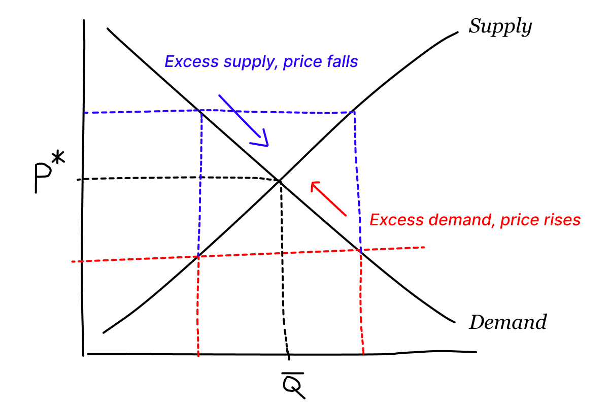
A numerical simulation can find $p^*$ by starting with a trial price, increasing it when demand exceeds supply, and decreasing it when demand is below supply. The search stops when total demand is sufficiently close to $\bar{Q}$. This means the market clears when neither excess demand nor excess supply remains:

$$\text{total demand} = \text{total permit supply}$$

The market-clearing price is therefore the price that makes all household decisions compatible with the regulator's fixed water cap.

---

8. Why the benchmark allocation is efficient

At the market-clearing price, every household with positive water consumption chooses:

$$MB_i(q_i^*)=p^*$$

This means that all active households have the same marginal benefit from the final unit of water they consume.

If one permit were moved from one active household to another, the benefit gained by the receiver would be offset by the benefit lost by the giver. No further transfer could increase total modeled benefit.

Equivalently, the market allocation solves the theoretical planner's problem:

$$\max_{\{q_i\}_{i=1}^{N}} \sum_{i=1}^{N}A_i\ln(q_i+1)$$

subject to:

$$\sum_{i=1}^{N}q_i=\bar{Q}$$

Under the benchmark assumptions, the permit market therefore allocates the fixed water supply efficiently in the narrow sense of maximizing total modeled benefit.

---

9. Determining the buyer and seller

Finding the market-clearing price tells us how much water each household wants to consume. The next step is to compare that desired amount with the number of permits the household originally received.

Let:

$$e_i$$

be household $i$'s initial permit allocation.

After finding the market-clearing price, household $i$ wants to consume:

$$q_i^*(p^*)$$

The difference between these two amounts is the household's net trade:

$$t_i=q_i^*(p^*)-e_i$$

if the net trade is positive:

$$t_i>0$$

the household wants more permits than it owns, so it buys permits.

if the net trade is negative:

$$t_i<0$$

the household owns more permits than it wants to use, so it sells permits.

And if the net trade is 0:

$$t_i=0$$

the household already owns exactly the number of permits it wants, so it neither buys nor sells.

Trading changes who holds the permits, but it does not change the total number of permits or the total amount of water allowed by the regulator.

So every permit purchased by one household must be sold by another household, total net trade across the market must equal zero:

$$\begin{aligned} \sum_{i=1}^{N}t_i &= \sum_{i=1}^{N} \left[q_i^*(p^*)-e_i\right]\\ &= \sum_{i=1}^{N}q_i^*(p^*) - \sum_{i=1}^{N}e_i\\ &= \bar{Q}-\bar{Q}\\ &=0. \end{aligned}$$

Therefore:

$$\text{total permits bought} = \text{total permits sold}$$

---

10. Model boundaries

The model is intentionally simple. The following problems are not generated inside the benchmark model because they are excluded by assumption.

Every household is assumed to be a price-taker, so the model does not account for market power. In a real market, one participant or a coordinated group might accumulate enough permits to influence prices or withhold supply.

Financial distress is also outside the model. There is no household income, debt, borrowing limit, or urgent need for cash, so it cannot represent a financially distressed household selling essential water permits to pay for other expenses.

The model does not impose a minimum quantity for basic water requirements. It allows:

$$q_i^*(p)=0$$

when the permit price is sufficiently high relative to $A_i$, even though households need some water for drinking, cooking, and hygiene.

Transaction costs and unequal access are excluded because trading is assumed to be immediate and free. A real system may involve fees, delays, limited information, or unequal access to the market.

Uncertainty is excluded by the model's one-period structure. Households know their valuation and do not need to reserve permits for emergencies or future water needs.

Strategic and speculative behavior is excluded as well. Households trade only to reach their preferred consumption. They do not withhold permits, manipulate the market, bank permits, or purchase them solely for resale.

---

Conclusion

A tradable water permit system combines a fixed environmental limit with decentralized household decisions. The regulator controls total water use by fixing the number of permits. Each household chooses its water consumption by comparing the marginal benefit of water with the permit price. The market-clearing price is the price at which total household demand equals the fixed permit supply.

At that price, households whose desired consumption exceeds their initial allocation buy permits, while households whose desired consumption is below their allocation sell permits. Total purchases equal total sales.

Under the benchmark assumptions, trading moves permits toward households with higher marginal benefits and maximizes the total benefit represented by the model.

The model should not be interpreted as proof that a real water market would be fair, safe, or desirable. It excludes income constraints, basic water requirements, market power, uncertainty, transaction costs, and strategic behavior.

The deeper question is not only whether a market can clear, but which protections and institutions would be required before such a market could protect basic water access and avoid exploitation.

---

References

1. [1]R. Quentin Grafton, Gary Libecap, Samuel McGlennon, Clay Landry, and Bob O'Brien (2011). An Integrated Assessment of Water Markets: A Cross-Country Comparison. Journal. ↩
2. [2]Xinchen Hu, Yu Li, Yan Sun, Chi Zhang, Wei Ding, and Jiahui Deng (2022). Water permits trading framework for urban water demand management based on smart metering. Journal. ↩
3. [3]W.David Montgomery (1972). Markets in licenses and efficient pollution control programs. Journal. ↩
4. [4]J.M. Dalhuisen, R.J.G.M. Florax, H.L.F. de Groot, and P. Nijkamp (2003). Price and Income Elasticities of Residential Water Demand: A Meta-Analysis. Journal. ↩
5. [5]Arnaud Reynaud, and Giulia Romano (2003). Price and Income Elasticities of Residential Water Demand: A Meta-Analysis. Journal. ↩